“If you torture the data long enough, it will confess to anything”
- Ronald Coase
In my last post, I briefly mentioned p-hacking in my discussion of how many social science papers are unreliable, and how terrible research practices partially underlie the sorry state of the literature. In this post, I want to describe “p-hacking” in greater detail and illustrate the concept by doing some p-hacking myself.
p-values, explained
If you haven’t taken a statistics course or it’s been a while, you might have forgotten what a p-value is in the first place (or never learned, which is also fine!). Here is a quick refresher.
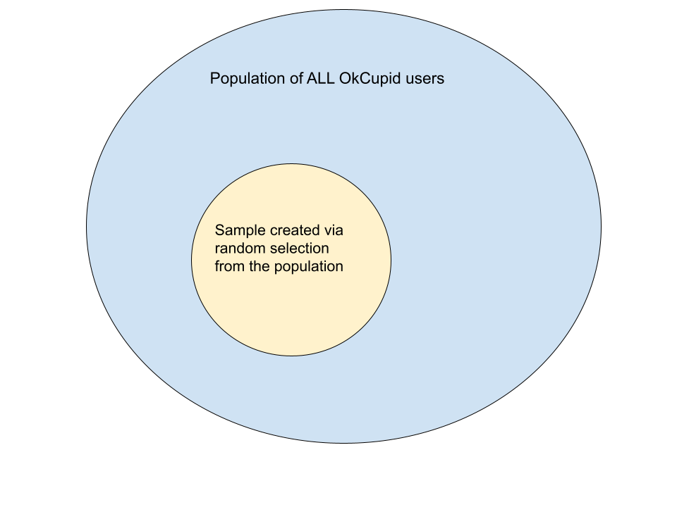
The p-value of a statistical test is the probability of obtaining a false positive result (i.e., a result that seems significant, but isn’t). To illustrate the concept, imagine you are a researcher analyzing this dataset of ~60 thousand OkCupid profiles.1 Let’s assume this is a representative sample of the population of all OkCupid users:
Sample (our dataset) vs. population of all OkCupid profiles.
Suppose you want to determine whether the average age of male and female OkCupid users is meaningfully different.
Your first instinct might be to simply… find the average age by gender and compare. And huzzah! The numbers are different:
  sex   mean_age
  <chr>    <dbl>
1 f         32.8
2 m         32.0
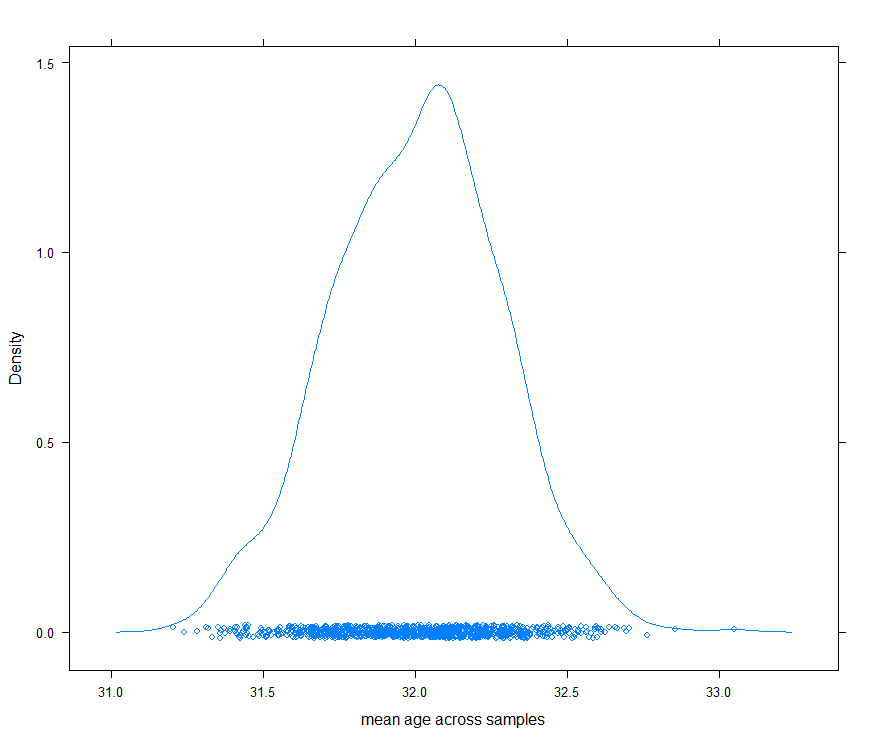
Unfortunately, it’s not that simple. Top-line statistics can be numerically different without indicating a statistically significant difference due to random variation in the specifics of a given sample. To illustrate, suppose I create 1,000 sub-samples from the initial 60 thousand-large dataset (each consisting of 1,000 male profiles selected at random). Here is the distribution of average male age across the samples:
As you can see, each particular sample has a slightly different sample mean (i.e., the average (of age in this case) for a sample drawn from a larger population).
The theoretical distribution of potential sample means is called the sampling distribution, and in the case of the mean for a normally-distributed population, it looks an awful lot like what I created above (i.e. bell-shaped).2
Before returning to p-values in particular, I want to explain another topic that will frame the p-value discussion: hypothesis testing.
Hypothesis testing
Let’s return to the initial research question: whether male OkCupid users are (on average) older or younger than female users (i.e., whether there is a statistically meaningful difference in the average age of male and female users).
For a hypothesis test in statistics, one establishes a “null hypothesis” that says there is not a significant difference/effect. With hypothesis testing, you assume that there is no such difference between the means (or, in the case of a regression coefficient, that the coefficient is not meaningfully different from 0). In this example, the null hypothesis H_0 would be:
H_0: mean_age_male = mean_age_female
With hypothesis testing, you start by assuming the null hypothesis is true. So in this case, you would assume that the average age of male OkCupid users comes from the same sampling distribution as the mean age of female users.
We then “test” this hypothesis by seeing how likely it is that both means do in fact come from the same sampling distribution. If this seems unlikely, we reject the null hypothesis and accept the alternative (which is the logical complement of the null). In this case, the alternative hypothesis H_1 would be that the mean age of female OkCupid users is not equal to the mean age of male users):
H_1: mean_age_male ≠ mean_age_female
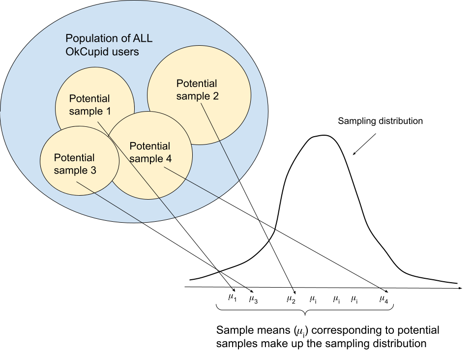
To recap: we can think of the sample mean as falling somewhere on a theoretical distribution of all potential sample means called the sampling distribution. In case it helps, here’s a diagram I made (with the m-looking greek letter mu the sample mean for a given sample i (so, mu_1 corresponds to potential sample 1, mu_2 corresponds to potential sample 2, etc.).
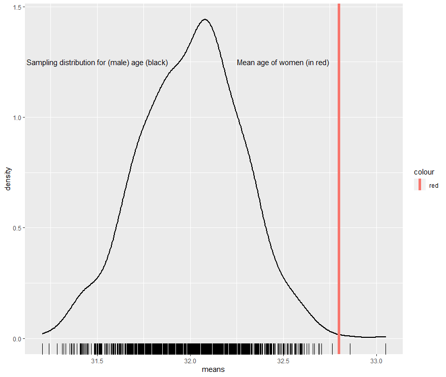
To determine whether to reject the null hypothesis, first imagine the average age of females is situated on the male sampling distribution (which is what we are saying with the null hypothesis). We then find the number of standard deviations the average age of females is from the center of the distribution.3 Here is where the mean age of females falls on the male sampling distribution:
Here is the information we need to calculate the number of standard deviations the mean age of females is from the mean age of men (which is our test statistic, t):
  sex   mean_age sd_age     n
  <chr>    <dbl>  <dbl> <int>
1 f         32.8  10.0  24117
2 m         32.0   9.03 35829
The formula for an unequal variances t-test
We find that t is approximately 10. Ten standard deviations out on the distribution! As a result, the p-value (the probability we obtained a false positive result, i.e. the probability our test statistic actually does come from the null distribution) is minute (<2.2e-16), and well below the 0.05 threshold typically used to define “statistical significance.” So we reject the null hypothesis in favor of the alternative hypothesis, that the mean age of female OkCupid users is meaningfully different from the mean age of male OkCupid users.
p-hacking, explained
P-values provide valuable information about the statistical significance of a difference in means (such as in the example above) or the effect of an independent variable on a dependent variable in the case of regression analysis. Unfortunately, p-values are easily-abused because they are calculated with the assumption that statistical tests are conducted one by one rather than repeatedly until the researcher obtains a “significant” result.
Many researchers compare numerous variables simultaneously in the hopes that one or more relationships are significant. And they do so without correcting for multiple comparisons (which is required due to the single-test assumption). Researchers also sometimes try to expand their sample until they reach significance. From this overview of p-hacking:
A lot of pressure rests on researchers to produce statistically significant results. For many researchers, statistical significance is the cornerstone of their academic career…
Now, what does a researcher do confronted with messy, non-significant results? According to several much-cited studies (for example John et al., 2012; Simmons et al., 2011), a common reaction is to start sampling again (and again, and again, …) in the hope that a somewhat larger sample size can boost significance. Another reaction is to wildly conduct hypothesis tests on the existing sample until at least one of them becomes significant (see for example: Simmons et al., 2011; Kerr, 1998 ). These practices, along with some others, are commonly known as p-hacking, because they are designed to drag the famous p-value right below the mark of .05 which usually indicates statistical significance. Undisputedly, p-hacking works (for a demonstration try out the p-hacker app).
…
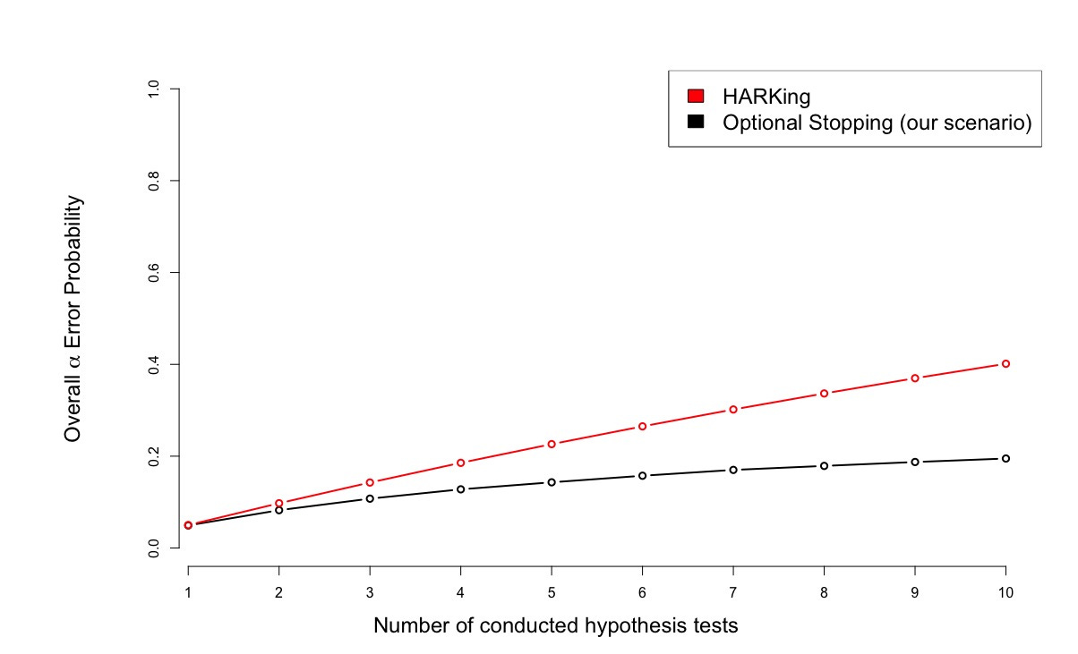
As a showcase, we want to introduce two researchers: The HARKer takes existing data and conducts multiple independent hypothesis tests (based on multiple uncorrelated variables in the data set) with the goal to publish the ones that become significant. For example, the HARKer tests for each possible correlation in a large data set whether it differs significantly from zero. On the other hand, the Accumulator uses optional stopping. This means that he collects data for a single research question test in a sequential manner until either statistical significance or a maximum sample size is reached.
…
We can see that HARKing produces higher false positive rates than optional stopping with the same number of tests. This can be explained through the dependency on the first sample in the case of optional stopping: Given that the null hypothesis is true, this sample is not very likely to show extreme effects in any direction (however, there is a small probability that it does). Every extension of this sample has to “overcome” this property not only by being extreme in itself but also by being extreme enough to shift the test on the overall sample from non-significance to significance. In contrast, every sample in the multiple testing case only needs to be extreme in itself.
To illustrate the ease with which one can obtain a fake result, I will randomly generate data and find significant relationship between my made-up variables. If you want to try this for yourself, I recommend checking out this p-hacking demo.
For this example, suppose we are studying the predictors of cognitive ability, and imagine our dependent variables y1, y2, and y3 (which are meant to measure cognitive ability, the outcome of interest) are IQ, SAT score, and GRE score. Suppose we have a sample size of 100 and randomly generate data for y1, y2, and y3 as follows:
# y (IQ)
# normally distributed with a mean of 100 and a standard deviation of # 15
y1 = rnorm(100,mean=100,sd=15)

# SAT
# normally distributed with a mean of 1051 and a standard deviation
# of 211
y2 = rnorm(100,mean=1051,sd=211)

# GRE
# normally distributed with a mean of 150 and a standard deviation of # 9
y3 = rnorm(100,mean=150,sd=9)
And suppose we randomly generate data for ten regressors, x1, x2, …, x10:
And voila! We have found a statistically significant relationship (under p<0.05 criteria) between x3 and y1 (IQ), with a respectable p-value4 of 0.0103. And we also found a just barely-insignificant relationship between x8 and y1.
This isn’t surprising: under p < 0.05 significance criteria, each time an independent variable is regressed against the dependent variable there is a 5% chance of obtaining a spurious relationship (1-0.95=0.05). So in the case of ten dependent variables, the probability of obtaining at least one false positive is about 40% (1-(0.95)^10 = 0.401).
Yet many seemingly-upstanding researchers would take the above results and write about the relationship between x3 and y1 without mentioning the insignificant p-values for the other regressors. Indeed, the studies cited in the quote above (John et al. (2012) and Simmons et al. (2011)) testify to the stunning prevalence of p-hacking techniques and other shady research methods. In their survey of nearly 6,000 academic psychologists, John et al. (2012) find that, for the “Bayesian-truth-serum (BTS) condition” (one portion of respondents had their answers run through a scoring algorithm “used to provide incentives for truth telling”):5
[N]early 1 in 10 research psychologists has introduced false data into the scientific record and…the majority of research psychologists have engaged in practices such as selective reporting of studies, not reporting all dependent measures, collecting more data after determining whether the results were significant, reporting unexpected findings as having been predicted, and excluding data post hoc.
This article is getting to be a bit long, so I’ll save further discussion of p-hacking and other questionably research practices for another post. I hope this article gave you a better understanding of p-values, why p-hacking is so disturbingly easy, and the frightening ubiquity of p-hacking techniques (and thus unreliable research!).
The sampling distribution is bell-shaped but not normally-distributed. Rather it is t-distributed. The t-distribution is similar to the normal distribution but has “fatter” tails:
In the regression output above, p-values are listed in the right-hand column (under “Pr(>|t|)”, and the dots and stars indicate the presence and magnitude of statistical significance (the “Signif. codes” row shows what the stars and dots indicate).
“[R]espondents were told that we would make a donation to a charity of their choice, selected from five options, and that the size of this donation would depend on the truthfulness of their responses, as determined by the BTS scoring system” (John et al. 2012, at p. 526). Note: the quoted passage below this footnote has been lightly edited for clarity.